
The fst package uses LZ4 and ZSTD to compress columnar data. In the latest release, methods compress_fst and decompress_fst were added which allow for direct (multi-threaded) access to these excellent compressors.
Table of Contents
LZ4 and ZSTD
LZ4 is one of the fastest compressors around, and like all LZ77-type compressors, decompression is even faster. The fst package uses LZ4 to compress and decompress data when lower compression levels are selected (in method write_fst). For higher compression levels, the ZSTD compressor is used, which offers superior compression ratio’s but requires more CPU resources.
How to use LZ4 and ZSTD from the fst package
From version 0.8.0, methods compress_fst and decompress_fst are available in the package. These methods give you direct access to LZ4 and ZSTD. As an example of how they can be used, we download a 90 MB file from Kaggle and recompress it using ZSTD:
library(fst)

# you can download this file from https://www.kaggle.com/stackoverflow/so-survey-2017
sample_file <- "survey_results_public.csv"

# read file contents into a raw vector
raw_vec <- readBin(sample_file, "raw", file.size(sample_file))

# compress bytes with ZSTD at a compression level of 20 percent
compressed_vec <- compress_fst(raw_vec, "ZSTD", 20)

# write the compressed data into a new file
compressed_file <- "survey_results_public.fsc"
writeBin(compressed_vec, compressed_file)

# compression ratio
file.size(sample_file) / file.size(compressed_file)
## [1] 8.949609
using a ZSTD compression level of 20 percent, the contents of the csv file are compressed to about 11 percent of the original size (calculated as the inverse of the compression ratio). To decompress the generated compressed file again you can do:
# read compressed file into a raw vector
compressed_vec <- readBin(compressed_file, "raw", file.size(compressed_file))

# decompress file contents
raw_vec_decompressed <- decompress_fst(compressed_vec)
A nice feature of data.table’s fread method is that it can parse in-memory data directly. That means that we can easily feed our raw vector to fread:
library(data.table)

# read data set from the in-memory csv
dt <- fread(rawToChar(raw_vec_decompressed))
This effectively reads your data.table from a compressed file, which saves disk space and increases read speed for slow disks.
Multi-threading
Methods compress_fst and decompress_fst use a fully multi-threaded implementation of the LZ4 and ZSTD algorithms. This is accomplished by dividing the data into (at maximum) 48 blocks, which are then processed in parallel. This increases the compression and decompression speeds significantly at a small cost to compression ratio:
library(microbenchmark)

threads_fst(8)  # use 8 threads

# measure ZSTD compression performance at low setting
compress_time <- microbenchmark(
  compress_fst(raw_vec, "ZSTD", 10),
  times = 500
)

# decompress again
decompress_time <- microbenchmark(
  decompress_fst(compressed_vec),
  times = 500
)

cat("Compress: ", 1e3 * as.numeric(object.size(raw_vec)) / median(compress_time$time), "MB/s",
    "Decompress: ", 1e3 * as.numeric(object.size(raw_vec)) / median(decompress_time$time), "MB/s")
## Compress: 1299.649 MB/s Decompress: 1948.932 MB/s
That’s a ZSTD compression speed of around 1.3 GB/s!
Bring on the cores
With more cores, you can do more parallel compression work. When we do the compression and decompression measurements above for a range of thread and compression level settings, we find the following dependency between speed and parallelism:
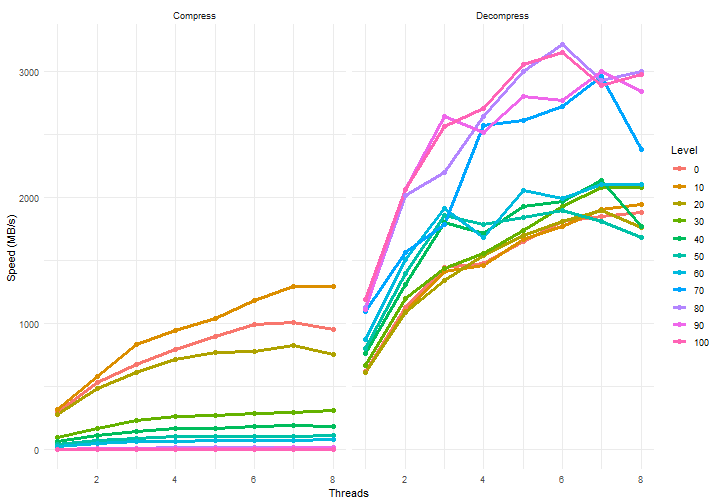 Figure 1: Compression and decompression speeds vs the number of cores used for computation
The code that was used to obtain these results is given in the last paragraph. As can be expected, the compression speed is highest for lower compression level settings. But interesting enough, decompression speeds actually increase with higher compression settings! For the highest levels, ZSTD decompression speeds of more than 3 GB/s were measured in our experiment!
Different compression levels settings lead to different compression ratio’s. This relation is depicted below. For completeness, LZ4 compression ratio’s were added as well:
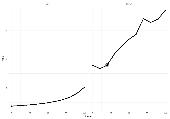 Figure 2: Compression ratio for different settings of the compression level
The highlighted point at a 20 percent (ZSTD) compression level corresponds to the measurement that we did earlier. It’s clear from the graph that with a combination of LZ4 and ZSTD, a wide range of compression ratio’s (and speeds) is available to the user.
The case for high compression levels
There are many use cases where you compress your data only once but decompress it much more often. For example, you can compress and store a file that will need to be read many times in the future. In that case it’s very useful to spend the CPU resources on compressing at a higher setting. It will give you higher decompression speeds during reads and the compressed data will occupy less space.
Also, when operating from a disk that has a lower speed than the (de-)compression algorithm, compression can really help. For those cases, compression will actually increase the total transfer speed because (much) less data has to be moved to or from the disk. This is also the main reason why fst is able to serialize a data set at higher speeds than the physical limits of a drive.
(Please take a look at this post to get an idea of how that works exactly)
Benchmark code
Below is the benchmark script that was used to obtain the dependency graph for the number of cores and compression level.
library(data.table)

# benchmark results
bench <- data.table(Threads = as.integer(NULL), Time = as.numeric(NULL),
  Mode = as.character(NULL), Level = as.integer(NULL), Size = as.numeric(NULL))

# Note that compression time increases steadily with higher levels.
# If you want to run this code yourself, start by using levels 10 * 0:5
for (level in 10 * 0:10) {
  for (threads in 1:parallel::detectCores()) {

    cat(".")  # show some progress
    threads_fst(threads)  # set number of threads to use

    # compress measurement
    compress_time <- microbenchmark(
      compressed_vec <- compress_fst(raw_vec, "ZSTD", level), times = 25)

    # decompress measurement
    decompress_time <- microbenchmark(
      decompress_fst(compressed_vec), times = 25)

    # add measurements to the benchmark results
    bench <- rbindlist(list(bench,
      data.table(
        Threads = threads,
        Time = median(compress_time$time),
        Mode = "Compress",
        Level = level,
        Size = as.integer(object.size(compressed_vec))),
      data.table(
        Threads = threads,
        Time = median(decompress_time$time),
        Mode = "Decompress",
        Level = level,
        Size = as.integer(object.size(compressed_vec)))))
  }
}
This creates a data.table with compression and decompression benchmark results.
This post is also available on R-bloggers

